Example Datasets

[1]:

import os
import warnings

os.environ["OMP_NUM_THREADS"] = "4"
os.environ["OPENBLAS_NUM_THREADS"] = "4"
os.environ["MKL_NUM_THREADS"] = "4"
os.environ["VECLIB_MAXIMUM_THREADS"] = "4"
os.environ["NUMEXPR_NUM_THREADS"] = "4"

from grnet.toydata import load_dataset, load_metadata
import matplotlib.pyplot as plt
import pandas as pd
from sklearn.manifold import TSNE

warnings.filterwarnings("ignore", category=RuntimeWarning, module="threadpoolctl")

Example datasets include followings: - Count data (\(\log_2(RPM+1)\)) - metadata

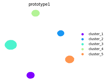
Prototype1

[2]:

data1 = load_dataset("prototype1")
meta1 = load_metadata("prototype1")

NxD matrix will be given (N: number of samples, D: number of genes)

[3]:

data1

[3]:

	gene_1	gene_2	gene_3	gene_4	gene_5	gene_6	gene_7	gene_8	gene_9	gene_10	...	gene_9991	gene_9992	gene_9993	gene_9994	gene_9995	gene_9996	gene_9997	gene_9998	gene_9999	gene_10000
sample_1	0.0	0.0	0.000000	0.0	0.000000	0.000000	0.000000	0.000000	0.000000	0.0	...	2.753703	0.000000	0.000000	0.000000	0.000000	10.273207	0.0	0.0	0.0	0.000000
sample_2	0.0	0.0	2.380056	0.0	0.000000	1.633563	9.828775	0.000000	0.000000	0.0	...	0.000000	2.869546	0.000000	4.155610	0.000000	9.673981	0.0	0.0	0.0	0.000000
sample_3	0.0	0.0	0.000000	0.0	0.000000	0.000000	0.000000	0.000000	0.000000	0.0	...	0.000000	0.000000	0.000000	2.083379	0.000000	9.719177	0.0	0.0	0.0	0.000000
sample_4	0.0	0.0	0.000000	0.0	0.000000	0.000000	0.000000	0.000000	3.832107	0.0	...	8.609340	6.330085	0.000000	0.000000	3.939771	10.232104	0.0	0.0	0.0	0.000000
sample_5	0.0	0.0	0.000000	0.0	0.000000	0.000000	0.000000	3.034451	0.000000	0.0	...	0.000000	0.000000	0.000000	0.000000	0.000000	10.091159	0.0	0.0	0.0	0.000000
...	...	...	...	...	...	...	...	...	...	...	...	...	...	...	...	...	...	...	...	...	...
sample_996	0.0	0.0	0.000000	0.0	0.000000	0.000000	0.000000	0.000000	3.380126	0.0	...	0.000000	0.000000	0.000000	0.000000	0.000000	0.000000	0.0	0.0	0.0	2.048660
sample_997	0.0	0.0	0.000000	0.0	0.000000	0.000000	0.000000	2.194422	0.000000	0.0	...	0.000000	0.000000	4.489439	0.000000	0.000000	0.000000	0.0	0.0	0.0	3.552277
sample_998	0.0	0.0	0.000000	0.0	8.068697	0.000000	0.000000	0.000000	0.000000	0.0	...	0.000000	0.000000	0.000000	0.000000	0.000000	0.000000	0.0	0.0	0.0	4.741316
sample_999	0.0	0.0	0.000000	0.0	1.796236	0.000000	2.571982	0.000000	0.000000	0.0	...	0.000000	0.000000	0.000000	0.000000	3.740458	0.000000	0.0	0.0	0.0	3.985389
sample_1000	0.0	0.0	0.000000	0.0	0.000000	0.000000	0.000000	0.000000	0.000000	0.0	...	0.000000	7.084269	0.000000	0.000000	0.000000	0.000000	0.0	0.0	0.0	9.423962

1000 rows × 10000 columns

in metadata, cluster info. is provided

[4]:

meta1

[4]:

	cluster
sample_1	1
sample_2	1
sample_3	1
sample_4	1
sample_5	1
...	...
sample_996	5
sample_997	5
sample_998	5
sample_999	5
sample_1000	5

1000 rows × 1 columns

Visualization

[5]:

# dimensionality reduction with TSNE

tsne1 = pd.DataFrame(
    TSNE(n_components=2, random_state=0).fit_transform(data1),
    index = data1.index,
    columns = [f"TSNE{i + 1}" for i in range(2)]
)

[6]:

fig, ax = plt.subplots(figsize=(4, 4))

for i, v in enumerate(meta1.cluster.unique()):
    _dat = tsne1[meta1.cluster == v]

    plt.scatter(
        _dat.iloc[:, 0], _dat.iloc[:, 1],
        color = plt.cm.rainbow(
            i / len(meta1.cluster.unique())
        ),
        label = f"cluster_{v}"
    )

ax.legend(loc="center left", bbox_to_anchor=(1, .5), frameon=False)
ax.axis("off")
ax.set(title="prototype1");

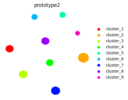
../_images/notebooks_example_data_11_0.png

Prototype2

[7]:

data2 = load_dataset("prototype2")
meta2 = load_metadata("prototype2")

[8]:

data2

[8]:

	gene_1	gene_2	gene_3	gene_4	gene_5	gene_6	gene_7	gene_8	gene_9	gene_10	...	gene_9991	gene_9992	gene_9993	gene_9994	gene_9995	gene_9996	gene_9997	gene_9998	gene_9999	gene_10000
sample_1	0.000000	3.507129	0.000000	0.000000	0.0	0.000000	0.0	0.0	0.0	0.000000	...	0.000000	0.000000	3.507129	0.000000	0.00000	0.0	8.004430	0.000000	0.000000	0.000000
sample_2	0.000000	0.000000	0.000000	0.000000	0.0	1.715359	0.0	0.0	0.0	0.000000	...	0.000000	2.477047	4.707172	0.000000	2.97294	0.0	8.314904	0.000000	0.000000	0.000000
sample_3	4.567996	0.000000	0.000000	0.000000	0.0	0.000000	0.0	0.0	0.0	0.000000	...	0.000000	0.000000	4.567996	1.941078	0.00000	0.0	7.904205	0.000000	0.000000	0.000000
sample_4	0.000000	0.000000	0.000000	0.000000	0.0	0.000000	0.0	0.0	0.0	0.000000	...	0.000000	0.000000	4.320645	0.000000	0.00000	0.0	8.602809	0.000000	0.000000	0.000000
sample_5	0.000000	8.222258	0.000000	0.000000	0.0	0.000000	0.0	0.0	0.0	0.000000	...	0.000000	0.000000	4.526527	0.000000	0.00000	0.0	7.378120	0.000000	0.000000	0.000000
...	...	...	...	...	...	...	...	...	...	...	...	...	...	...	...	...	...	...	...	...	...
sample_1496	3.786429	0.000000	0.000000	0.000000	0.0	0.000000	0.0	0.0	0.0	0.000000	...	0.000000	3.169765	0.000000	0.000000	0.00000	0.0	0.000000	0.000000	8.647279	1.378401
sample_1497	6.193268	0.000000	0.000000	0.000000	0.0	0.000000	0.0	0.0	0.0	0.000000	...	0.000000	0.000000	0.000000	0.000000	0.00000	0.0	3.366368	0.000000	10.656825	0.000000
sample_1498	6.028006	3.371017	0.000000	3.001727	0.0	0.000000	0.0	0.0	0.0	0.000000	...	0.000000	0.000000	0.000000	0.000000	0.00000	0.0	3.371017	0.000000	10.925548	0.000000
sample_1499	5.144795	0.000000	1.595626	2.821051	0.0	0.000000	0.0	0.0	0.0	8.670563	...	2.334715	0.000000	0.000000	0.000000	0.00000	0.0	3.473954	3.715184	9.994661	0.000000
sample_1500	4.536216	0.000000	0.000000	0.000000	0.0	0.000000	0.0	0.0	0.0	0.000000	...	0.000000	0.000000	0.000000	0.000000	0.00000	0.0	4.205152	0.000000	9.952163	0.000000

1500 rows × 10000 columns

[9]:

meta2

[9]:

	cluster
sample_1	1
sample_2	1
sample_3	1
sample_4	1
sample_5	1
...	...
sample_1496	9
sample_1497	9
sample_1498	9
sample_1499	9
sample_1500	9

1500 rows × 1 columns

Visualization

[10]:

# dimensionality reduction with TSNE

tsne2 = pd.DataFrame(
    TSNE(n_components=2, random_state=0).fit_transform(data2),
    index = data2.index,
    columns = [f"TSNE{i + 1}" for i in range(2)]
)

[11]:

fig, ax = plt.subplots(figsize=(4, 4))

for i, v in enumerate(meta2.cluster.unique()):
    _dat = tsne2[meta2.cluster == v]

    plt.scatter(
        _dat.iloc[:, 0], _dat.iloc[:, 1],
        color = plt.cm.hsv(
            i / len(meta2.cluster.unique())
        ),
        label = f"cluster_{v}"
    )

ax.legend(loc="center left", bbox_to_anchor=(1, .5), frameon=False)
ax.axis("off")
ax.set(title="prototype2");

../_images/notebooks_example_data_18_0.png